SAS Exponential Distribution Code Example

The Exponential distribution is a continuous probability distribution. It models the time between events. The events occur on average at a constant rate, i.e. a Poisson process. Here, events occur continuously and independently. It has Probability Density Function

$\begin{equation*} f(x) = \frac{1}{\sigma} \exp \left(- \frac{x}{\sigma} \right), \quad x \geq 0. \end{equation}$

However, often you will see the density defined as

$\begin{equation*} f(x) = \lambda e^{- \lambda x}, \quad x \geq 0. \end{equation}$

where $\lambda=\frac{1}{\sigma}$ . $\sigma$ is the scale parameter and $\lambda$ is the rate parameter. The rate parameter indicates the rate at which the event occurs. The two densities are the same, but since the SAS PDF function takes $\sigma$ as argument, I like to go with that one. If a stochastic variable $X$ is exponentially distributed, we write $X \sim Exp(\sigma)$ . We define the density to zero for $x<0$ .

The Exponential is a special case of the Gamma distribution with shape parameter $a=1$ and scale parameter $\lambda$ .

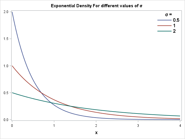
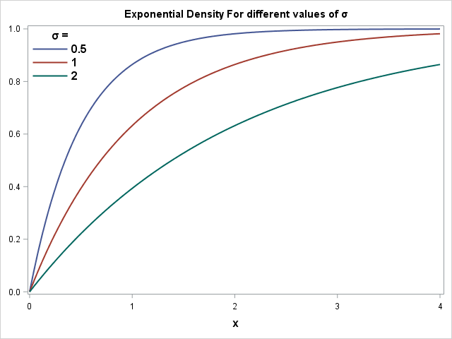
I plot the Probability Density Functions and the corresponding Cumulative Density Functions to the right. Here, I use different values of $\sigma$ . You can download the code creating these plots here.

Exponential Probability Density Function PDF

Exponential Cummulative Density Function CDF

SAS Code Example

The SAS code below lets you set $\sigma$ and draw the probability density function for the corresponding exponential function. I encourage you to play around with this code. Familiarize yourself with the impact of $\sigma$ on the shape of the density.

/* Exponential PDF Curves */
%let sigma = 1;
 
data Exponential_PDF;
         do x=0 to 4 by 0.01;
            Exponential_PDF = pdf('Exponential', x, &sigma);
            output;
         end;
run;
 
/* Draw PDF Curve */
title "Exponential Density For (*ESC*){unicode sigma} = &sigma";
proc sgplot data=Exponential_PDF noautolegend;
   series x=x y=Exponential_PDF / lineattrs = (thickness=2 color=black) legendlabel="Exponential PDF";
   keylegend / position=NE location=inside across=1 noborder valueattrs=(Size=12 Weight=Bold) 
                                 titleattrs = (Size=12 Weight=Bold);
   xaxis label='x' labelattrs = (size=12 weight=Bold);
   yaxis display=(nolabel) label='PDF' labelattrs = (size=12 weight=Bold);
run;
title;

Finally, check out the related pages about the Lognormal and Gamma Distribution in SAS.