SAS Negative Binomial Distribution Example

The Negative Binomial Distribution is a discrete probability distribution. It is a natural extension of the Poisson Distribution. It relaxes the assumption of equal mean and variance. The distribution has probability mass function

$\begin{equation*} P(X=k) = p(k) = {{n+k-1}\choose{k}} (1-p)^r p^k, \quad k=0, 1, 2, \dots \end{equation*}$

where ${{n+k-1}\choose{k}}$ is the binomial coefficient, explained in the Binomial Distribution. The Negative Binomial models the number of successes in a sequence of independent and identically distributed Bernoulli Trials (coinflips) before a specified (non-random) number of failures (denoted r) occurs.

Consequently, the Geometric Distribution is a special case of the Negative Binomial distribution with $n=1$ .

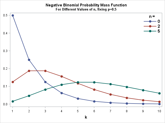
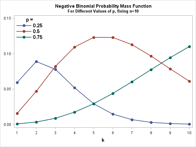
To the right, you can see Probability Mass Functions for different values of $n$ and $p$ respectively. You can download the code creating these plots here.

For a more thorough walkthrough of the distribution check out the YouTube video Introduction to the Negative Binomial Distribution by JbStatistics.

Negative Binomial Distribution Probability Mass Function PMF

Negative Binomial Probability Mass Function PMF

Negative Binomial SAS Code Example

Below, I have written a small SAS program that lets you set $n$ and $p$ and draw the corresponding Probability Mass Function. I encourage you to play around with the parameters. What happens when n is small? And can you make the negative binomial distribution look like a geometric distribution?

%let n=10;
%let p=0.5;
 
data negbin_PMF;
   do k=1 to 10;
      pmf=pdf('negbinomial', &n, &p, k);
      output;
   end;
run;
 
/* Draw PMF Curves */
title "Negative Binomial Probability Mass Function";
title2 "For Different n=&n, and p=&p";
proc sgplot data=negbin_PMF noautolegend;
   series x=k y=pmf / markers lineattrs=(thickness=2) markerattrs=(size=10 symbol=circlefilled);
   xaxis values=(1 to 10) labelattrs=(size=12 weight=Bold);
   yaxis display=(nolabel);
run;
title;

The negative binomial distribution models count data and is often used in cases where the variance is much greater than the mean. Consequently, these are the cases where the Poisson distribution fails.

Finally, I write about how to fit the negative binomial distribution in the blog post Fit Poisson and Negative Binomial Distribution in SAS.