Last week, I wrote the blog post Using the BUFSIZE and BUFNO System Options in SAS. Here, I introduced the two SAS system options BUFSIZE and BUFNO. The BUFSIZE Option controls the physical size of each data buffer, that SAS allocates for I/O operations in memory. The BUFNO System Option controls how many buffers SAS allocates.

Today, I will demonstrate the magnitude of increased performance with an example. There are many ways to measure performance. However, I will focus on elapsed time. Other reasonable measures could be I/O Operations, memory consumption, and so on. In the example to come, I use the SAS LOGPARSE macro to gather information from the study. See the post Track Performance in SAS with the LOGPARSE Macro for setup details.

Elapsed Time Example For Different Values of BUFSIZE and BUFNO

In the code below, I first create a data set a. Then I create a data set b, which reads from data set a. Consequently, I write to disk twice and read from disk once. I use CALL EXECUTE logic to repeat this for multiple values of BUFSIZE and BUFNO respectively.

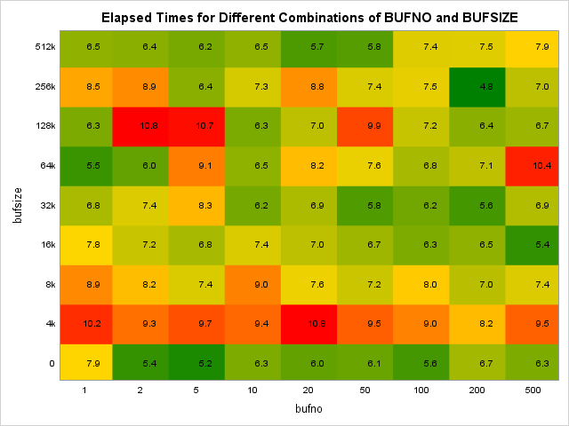
I have plotted the results from a run with 1Mio rows in each SAS data set. As a starting point, note that the default values for BUFZISE and BUFNO of 0 and 1 respectively are plotted in the southeast corner. This run takes 7.9 seconds. The plot reveals that while the default values do a decent job in this case, there are substantial gains in run time to be made. The best run takes place with 200 buffers and 256k in each buffer. It seems that for these data sets, it is beneficial to have more than 10 buffers and more than 16k allocated to each buffer. Remember though that it is memory costly to increase values to these points. Note that simply allocating one extra buffer, holding BUFSIZE=0 yields a sizable reduction in elapsed time as well. This is less memory costly than increasing BUFNO and BUFSIZE further.

options fullstimer;
options msglevel=i;
 
options nonotes nosource;
proc printto log="c:\Users\Peter\Desktop\MyLog.log";
run;
options notes source;
 
%passinfo;
 
data callstack;
   length string $500;
   do bufsize=0, 4, 8, 16, 32, 64, 128, 256, 512;
      do bufno=1, 2, 5, 10, 20, 50, 100, 200, 500;
         string=compbl(cats(
            "
            data a(bufsize=", bufsize, "k bufno=", bufno, ");
               length string $1000;
               do x=1 to 10e5;
                  output;
               end;
            run;
 
            data b(bufsize=", bufsize, "k bufno=", bufno, ");
               set a;
            run;
            "
            ));
         output;
         call execute(string);
      end;
   end;
run;
 
proc printto;
run;
 
%logparse(c:\Users\Peter\Desktop\MyLog.log,PerfStat,,,append=NO);

The above plot points out the benefits of increasing BUFNO and BUFSIZE. However, you should always thoroughly run tests on your actual data in your actual environment to make good choices about system options like these. Far too many factors influence performance statistics to rely on other people’s results.

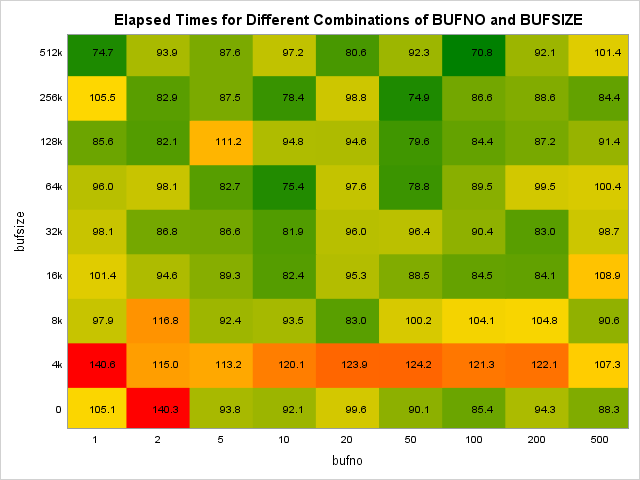
As an example, I have plotted the results for the same run as above, but with 10Mio observations instead of 1Mio. While we saw that we could benefit from simply changing BUFNO from 1 to 2 before, it is definitely not the case here. In this example, we see a clear increase in elapsed time for 2 buffers instead of one. However, from 5 buffers and above, we start to see performance gains.

Summary

When you read or write large amounts of data between disk and memory, you should consider how to allocate the buffers that hold the data in memory. In this post, we have seen the impact of the SAS BUFSIZE and BUFNO options. While we saw good results in terms of elapsed time here, it is not necessarily the case. Always do thorough testing on your own data and in your own environment.

As a related post, check out how to use the SASFILE Statement to Load a Data Set Into Memory.

You can download the entire code from this example here. The code in the link contains the graphing code as well.