In the blog post Fit Distribution to Continuous Data in SAS, I demonstrate how to use PROC UNIVARIATE to assess the distribution of univariate, continuous data. While PROC UNIVARIATE handles continuous variables well, it does not handle the discrete cases. Consequently, we need some other method if we wish to fit some theoretical distribution to discrete univarate data. In this post, I show an example of how to fit two common discrete distributions to the same univariate data and assess the best fitting distribution with PROC GENMOD.

The Data

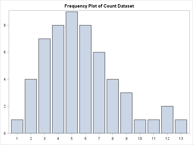
First of all, let us create some small, simple count dataset and look at how the data is distributed using a simple plot.

data CountData;
input count @@;
datalines;
   5 8 5 6 3 3 6 4 8 9 5 2 6 6 6 3 6 7 5 4 1 7 7 6 5 5
   4 4 4 4 5 8 8 5 9 10 4 9 5 3 7 6 13 2 4 12 11 12
   7 7 2 3 2 3 3
;

Visually, it seems like the data could be fitted well by a simple discrete distribution. Let us first take a look at fitting the data with the Poisson distribution.

Poisson Example

The Poisson Distribution is a very simple discrete probability distribution with a single parameter $\lambda$ , that represents both the mean and variance. I use PROC GENMOD to fit the Poisson distribution to the hypothetical data above. In the model statement I specify the dependent variable count and no independent variables. At first, this may seem a bit odd. But remember that when no explanatory variables are specified, only the mean of the model is fitted, which is exactly what we want. I specify the dist=Poisson option to the model statement to emphasize that I want to fit the Poisson. Lastly, I output the fitted parameters to the PoissonFit dataset for later analysis.

/* Fit Poisson distribution to data. */
proc genmod data=CountData;
   model count= /dist=Poisson;       /* No variables are specified, only mean is estimated. */
   output out=PoissonFit p=lambda;
run;
 
/* Save Poisson parameter lambda in macro variables. */
data _null_;
   set PoissonFit(obs=1);
   call symputx('lambda', lambda);
run;
 
/* Use Min/Max values and the fitted Lambda to create theoretical Poisson Data. */
data TheoreticalPoisson;
   do count=&minCount to &maxCount;
      po=pdf('Poisson', count, &lambda);
      output;
   end;
run;

As a result, the above Genmod Procedure yields a highly significant Maximum Likelihood estimate of $\lambda=5.71$ . In the two datasteps following the Genmod Procedure, we save the ML estimate of $\lambda$ in a macro variable and calculate the theoretical Probability Mass Function of a Poisson distribution with this parameter for later comparison of the actual data and the fitted PMF.

Negative Binomial Example

The Negative Binomial Distribution is a discrete probability distribution, that relaxes the assumption of equal mean and variance in the distribution. Working with count data, you will often see that the variance in the data is larger than the mean, which means that the Poisson distribution will not be a good fit for the data.

/* Fit Negative Binomial distribution to data. */
proc genmod data=CountData;
   model count= /dist=NegBin;       /* No variables are specified, only mean is estimated */
   ods output parameterestimates=NegBinParameters;
run;
 
/* Transpose Data. */
proc transpose data=NegBinParameters out=NegBinParameters;
   var estimate;
   id parameter;
run;
 
/* Calculate k and p from intercept and dispersion parameters. */
data NegBinParameters;
   set NegBinParameters;
   k = 1/dispersion;
   p = 1/(1+exp(intercept)*dispersion);
run;
 
/* Save k and p in macro variables. */
data _null_;
   set NegBinParameters;
   call symputx('k', k);
   call symputx('p', p);
run;
 
/* Calculate theoretical Negative Binomial PMF based on fitted k and p. */
data TheoreticalNegBin;
   do count=&minCount to &maxCount;
      NegBin=pdf('NegBinomial', count, &p, &k);
      output;
   end;
run;

Similar to the Poisson example, I use PROC GENMOD to fit the model with no explanatory variables. Also, I specify the dist=negbin to fit a discrete Negative Binomial Distribution. After that, I calculate $k$ and $p$ from the ML estiamtes of the dispersion and intercept in the model. This results in ML estimates of $k=22.29$ and $p=0.80$ . Similar to the Poisson example, I save these in macro variables and use these to calculate the theoretical Probability Mass Function of a Negative Binomial distribution with the estimated parameters $k$ and $p$ .

Compare Fitted Distributions with Data

Finally, I Merge the Theoretical Poisson and Negative Binomial Probability Mass Functions with the original count data. Then I plot the count data overlaid with the fitted Poisson and Negative Binomial distribution. I use the VBARPARM statement because this way, I can overlay the plot with the scatterplots from the fitted PMFs.

/* Merge The datasets for plotting. */
data PlotData(keep=count freq po negbin);
   merge TheoreticalPoisson TheoreticalNegBin CountMinMax;
   by count;
   freq = PERCENT/100;
run;
 
/* Overlay fitted Poisson density with original data. */
title 'Count data overlaid with fitted distributions';
proc sgplot data=PlotData noautolegend;
   vbarparm category=count response=freq / legendlabel='Count Data';
   series x=count y=po / markers markerattrs=(symbol=circlefilled color=red) 
                         lineattrs=(color=red)legendlabel='Fitted Poisson PMF';
   series x=count y=NegBin / markers markerattrs=(symbol=squarefilled color=green) 
                             lineattrs=(color=green)legendlabel='Fitted Negative Binomial PMF';
   xaxis display=(nolabel);
   yaxis display=(nolabel);
   keylegend / location=inside position=NE across=1;
run;
title;

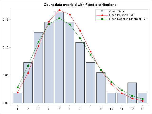
Visually, both the Poisson and Negative Binomial distribution seems to fit the data quite well. In addition, The discrete Negative Binomial seems to capture the skewness in the data better than the Poisson. This is supported by the Goodness of Fit statistics from the Genmod Procedure, which supports the visual conclusion, that the fitted Negative Binomial is the best fit to the data.

Summary

SAS can fit discrete probability distributions to univariate data with the Genmod Procedure. Needless to say, this is not the only way, but in my opinion it is the simplest and most efficient. You can also use PROC COUNTREG as demonstrated in this Example. As this example shows, fitting discrete distributions requires a bit more work than using PROC UNIVARIATE in the continuous case. You may wonder why we use PROG GENMOD or PROC QUANTREG to univariate analysis, because these are traditional regression procedures. I certainly did when I first learned about this. For a great introduction to why this is a very good idea in SAS, check out the article Use regression for a univariate analysis? Yes! by Rick Wicklin.

Finally, you can download the entire program from this post here.

Fit Discrete Distribution in SAS

The Data

Poisson Example

Negative Binomial Example

Compare Fitted Distributions with Data

Summary