SAS Fit Normal and Lognormal Distribution

One of the most important questions preceding most statistical analyses is “How is my data distributed?”. It is important to know your data well and also to be certain about the distribution of your data. Therefore, you should familiarize yourself with the different tools available for distribution fitting. Remember that univariate simply means ‘one variable’. Here, I will present the most common way to fit the Normal, Weibull and Lognormal in SAS with a PROC UNIVARIATE example.

PROC UNIVARIATE

When we examine the distribution of continuous univariate data, the first procedure that should come to mind is PROC UNIVARIATE. I usually assess the distribution of my data using these three tools:

Histogram – Plotting an empirical histogram of your data and overlaying it with the best fitting theoretical densities of the distributions you wish to assess is usually the first line of business. As a result, it gives you a nice visual overview of what distributions may fit your data well.
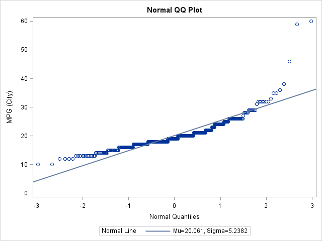
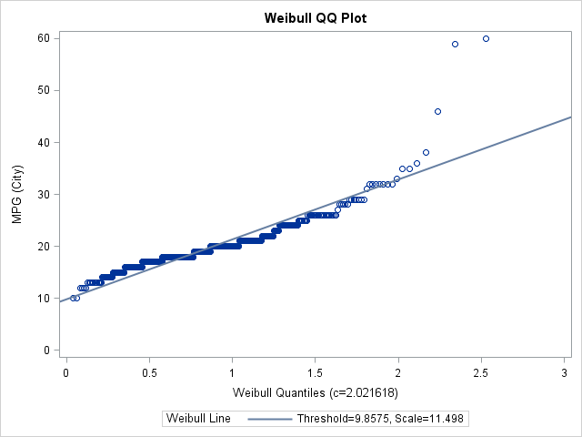
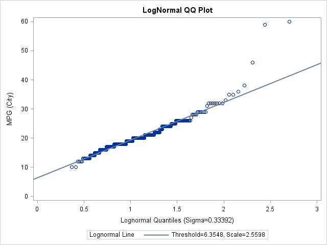
QQ Plot – The Quantile-Quantile plot compares ordered variable values with quantiles of some known theoretical distribution. If the theoretical distribution fits the data well, the QQ plot will form a linear pattern of points.
Goodness of Fit Test – The Histogram and QQ Plot are great tools to visually assess the distribution of your data. Goodness of Fit tests are statistical sizes that quantify how well some distribution fits your data.

An Example

Let us look at an example with the Miles Pr Gallon in the City variable (mpg_city). I use the Sashelp.Cars dataset and the Ods Select Statement to select only the three pieces of output from above.

ods select Histogram QQplot GoodnessOfFit;               /* Select only the relevant output  */
proc univariate data=sashelp.cars;
   histogram mpg_city/ normal
                       weibull(theta=est)                /* Default is theta = 0.            */ 
                       lognormal(theta=est)
                       midpoints = 4 to 62 by 2
                       odstitle = "Assesing Distribution Using Proc Univariate";
   qqplot mpg_city / normal(mu=est sigma=est) odstitle = "Normal QQ Plot.";
   qqplot mpg_city / weibull(c=est sigma=est theta=est) odstitle = "Weibull QQ Plot.";
   qqplot mpg_city / lognormal(sigma=est theta=est zeta=est) odstitle = "LogNormal QQ Plot.";
run;

Histogram

First of all, I use the HISTOGRAM statement in the above procedure with the Normal, Weibull and Lognormal options to request a histogram of the mpg_city variable overlaid with fitted densities from the Normal, Weibull and Lognormal using Maximum Likelihood estimation. Then, I use the theta=est option to suppress the default option of theta=0 and tell SAS to estimate the threshold parameter $\theta$ as well. The histogram is seen to the right. Visually, it seems like the lognormal fits our data the best because it describes both the peak and the skewness of the data.

QQ Plots

After looking at the histogram, I also request the QQ-plots for the same three distributions as specified in the histogram. Here though, the syntax does not allow me to request these in a single statement. Therefore, I have to use three distinct statements. The QQ-plots from PROC UNIVARIATE below supports the visual evidence that the data is Lognormally distributed since the Lognormal plot seems to resemble the linear reference line the best.

Goodness Of Fit Tests

Finally, we look at the Goodness of Fit Statistics for the three distributions. Implicitly, we request these with the Histogram Statement. These suggest that the Lognormal distribution fits the data the best of the three distributions.

Summary

PROC UNIVARIATE handles continuous variables only. You can not fit discrete probability distributions to univariate data such as Poisson or Negative Binomial with the Univariate Procedure. To see an example of how to fit discrete data, see the article Fit Poisson And Negative Binomial Distribution In SAS. For code examples of the three distributions assessed in the above PROC UNIVARIATE example and many more, check the Distribution Examples under the Examples menu, where I present code examples of the Normal, Weibull and Lognormal.

You can download the entire program from this post here.

Fit Continuous Distribution in SAS