Gamma Distribution Code Example in SAS

The Gamma Distribution is a continuous probability distribution. It is a two parameter distribution defined in terms of $\lambda$

and $a$

. We call these the scale and shape parameter of the distribution respectively. A random variable is Gamma distributed if it has the following probability density function.

$\begin{equation*} P(X=x) = p(x) = \frac{1}{\Gamma(a) \lambda^a} x^{a-1} \exp \left(- \frac{x}{\lambda} \right). \end{equation*}$

Here $\Gamma$ is the Gamma function. When you browse various statistics books you will find that the probability density function for the Gamma distribution is defined in different ways. However, this is one of the most common definitions of the density. Furthermore, I choose to define the density this way because the SAS PDF Function also does so.

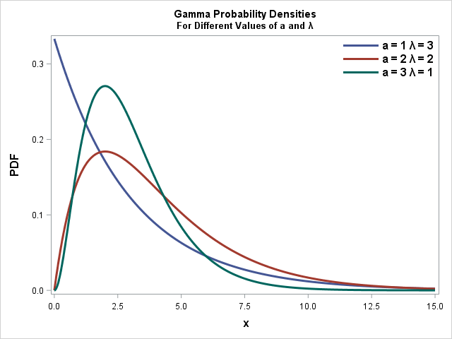
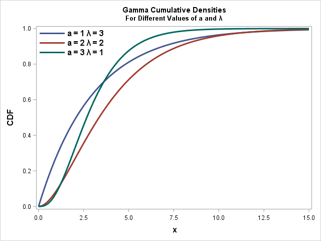
To the right, I have plotted densities and their corresponding cumulative Densities for three different Gamma distributions with different shape and scale parameters. You can download the program creating the plots here and insert into your own editor.

The Exponential Distribution is a special case of the Gamma distribution with shape parameter $a=1$ and scale parameter $\lambda$ .

Another special case of the Gamma distribution is the Chi-Squared Distribution with shape parameter $a=\frac{\nu}{2}$ and scale parameter $\lambda=1$ . That means that we can interpret a $\chi_n^2$ distribution with $n$ degrees of freedom as a $\Gamma \left( \frac{\nu}{2}, 2 \right)$ distribution.

Finally, I have previously written about how to Fit Continuous Distributions in SAS. Here, I write about fitting the Normal, Weibull and Lognormal distribution to univariate data. Needless to say, this method is also applicable for the Gamma distribution.

SAS Code Gamma Example

Below, I have written a small SAS program that lets you set the shape parameter $a$ and scale parameter $\lambda$ and plot the corresponding Gamma probability density function. Consequently, I encourage you to copy/paste this code into your editor and familiarize yourself with how the shape and scale parameters affect the distribution. What happens when both parameters are small? And what happens when one is much bigger than the other?

%let a=2;
%let lambda=2;
 
data PDF;
      do x=0 to 15 by 0.01;
         pdf=pdf('Gamma', x, &a, &lambda);
         output;
      end;
run;
 
title "Gamma Probability Densities.";
title2 "For Different Values of a=&a and (*ESC*){unicode lambda}=&lambda.";
proc sgplot data = PDF noautolegend;
   series x=x y=pdf/ lineattrs=(thickness=3) legendlabel="a = 1 (*ESC*){unicode lambda} = 3";
   yaxis label="PDF" labelattrs=(size=12 weight=Bold);
   xaxis label='x' labelattrs=(size=12 weight=Bold);
run;
title;