SAS Geometric Distribution Code Example

The geometric distribution is a discrete probability distribution. It models the probability that it takes exactly $k$

failures before we observe the first success in a series of independent Bernoulli Trials, each with success probability $p$

. The Probability Mass Function is given as

$\begin{equation*} P(Y=k) = p (1 - p)^k, \quad k \in \left{ 0, 1, 2, \dots \right}. \end{equation*}$

Here, $p$ is the probability of success and $k$ is the number of failures before the first success. Notice that k is allowed to be zero. $k=0$ means that you do not have to observe any failures before the first success, i.e. the first observation is a success. You may also see the Probability Mass Function defined as

$\begin{equation*} P(Y=k) = p (1 - p)^{k-1}, \quad k \in \left{ 1, 2, \dots \right}. \end{equation*}$

Here, $k$ is not allowed to be zero. Consequently $k=1$ means that you have to use 1 try to get the first success in this definition. Which definition you use is a matter of preference. I prefer the first one, since to me it makes most sense intuitively. Furthermore the SAS PDF Function interprets the Geometric Distribution this way.

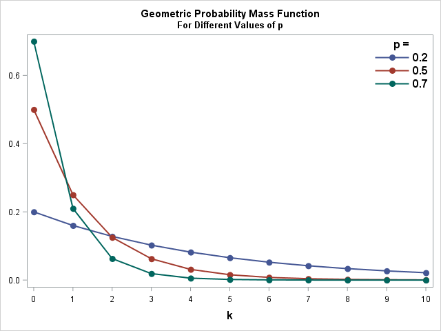
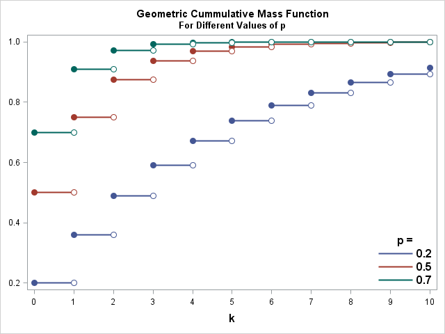
Obviously, the Probability Mass Function is strictly decreasing. You can see from the plotted Probability Mass Functions and corresponding Cumulative Mass Functions plotted to the right. Here, I have plotted three different PMF curves for three different values of $p$ . You can download the code to create these plots here.

The Geometric Distribution is a special case of the Negative Binomial Distribution. Recall that the Negative Binomial Distribution models the probability of the number of observing exactly $n$ failures before observing $k$ successes in a series of independent Bernoulli trials. Therefore, the Geometric Distribution is a special case of the Negative Binomial Distribution with $k=1$ . For a more thorough introduction to the Geometric distribution see the video An Introduction to the Geometric Distribution by jbStatistics.

Geometric SAS Code Example

Finally, I have written a small SAS program, that lets you set different values of success probability $p$ and plot the corresponding Probability Mass Function for the Geometric distribution. I encourage you to play around with this parameter. What happens when $p$ is very high? Or very low?

%let p=0.9;
 
/* Geometric Probability Mass Function Data */
data Geometric_PMF;
      do k=0 to 10;
         pmf=pdf('geometric', k, &p);
         output;
      end;
run;
 
/* Draw Geometric PMF Curve */
title "Geometric Probability Mass Function for p=&p";
proc sgplot data=Geometric_PMF noautolegend;
   series x=k y=pmf / markers lineattrs=(thickness=2) markerattrs=(size=10 symbol=circlefilled);
   xaxis values=(0 to 10) label='k' labelattrs=(size=12 weight=Bold);
   yaxis display=(nolabel);
   keylegend / titleattrs=(Size=12 Weight=Bold) 
               position=NE location=inside across=1 noborder valueattrs=(Size=12 Weight=Bold);
run;
title;