Using An Index to Increase Performance in SAS

Indexing data sets is an extremely powerful tool in SAS. It is also one of the most overlooked data manipulation features in SAS. Indexes are most powerful when you want to make a small subset of a large data set. Their usefulness reaches far beyond that though. This post provides a brief introduction to the concept of indexes and an example of how the index can reduce run time and increase performance in your programs, when used correctly. Furthermore, it gives me the opportunity to use one of my favorite procedures: PROC DATASETS.

First, let us create a large example data set. The data set contains 100 mio. rows and takes up about 7 GB disc space, so if you want a smaller data set, simply decrease the size of the do loop in the code.

data MyData;
   length ID 8 first_name $20 last_name $20 gender $1 state $20 birth_date 6 children 3;
 
   array first_namesm{20}$20 _temporary_ ("Paul", "Allan", "Bob", "Michael", "Chris", "David", "John", "Jerry", "James", "Robert",
                                       "William", "Richard", "Thomas", "Daniel", "Paul", "George", "Larry", "Eric", "Charles", "Stephen");
   array first_namesf{20}$20 _temporary_ ("Mary", "Linda", "Patricia", "Barbara", "Elizabeth", "Maria", "Susan", "Margaret", "Lisa", "Nancy",
                                       "Karen", "Betty", "Helen", "Sandra", "Sharon", "Laura", "Michelle", "Angela", "Melissa", "Amanda");
   array last_names{20}$20 _temporary_ ("Smith", "Johnson", "Williams", "Jones", "Brown", "Miller", "Wilson", "Moore", "Taylor", "Hall",
                                      "Anderson", "Jackson", "White", "Harris", "Martin", "Thompson", "Robinson", "Lewis", "Walker", "Allen");
   array states{50}$20 _temporary_ ("Alabama", "Alaska", "Arizona", "Arkansas", "California", "Colorado", "Connecticut", "Delaware", "Florida", 
                                "Georgia", "Hawaii", "Idaho", "Illinois", "Indiana", "Iowa", "Kansas", "Kentucky", "Louisiana", "Maine",
                                "Maryland", "Massachusetts", "Michigan", "Minnesota", "Mississippi", "Missouri", "Montana", "Nebraska", 
                                "Nevada", "New Hampshire", "New Jersey", "New Mexico", "New York", "North Carolina", "North Dakota", "Ohio", 
                                "Oklahoma", "Oregon", "Pennsylvania", "Rhode Island", "South Carolina", "South Dakota", "Tennessee", "Texas", 
                                "Utah", "Vermont", "Virginia", "Washington", "West Virginia", "Wisconsin", "Wyoming");
 
   call streaminit(123);
 
   do ID=1 to 10e7;
      if rand("Uniform")<0.5 then do;
         gender="M";
         first_name=first_namesm[ceil(rand("Uniform")*20)];
      end;
      else do;
         gender="F";
         first_name=first_namesf[ceil(rand("Uniform")*20)];
      end;
      last_name=last_names[ceil(rand("Uniform")*20)];
      state=states[ceil(rand("Uniform")*50)];
      birth_date=rand("Integer", '01jan1950'd, '01jan1990'd);
      children=rand("Table", 0.1, 0.2, 0.3, 0.2, 0.1, 0.1)-1;
      output; 
   end;
 
   format birth_date date9.;
run;

Create an Index with PROC DATASETS

When you create an index, it is stored in a file in the same location as the data set to which it relates. The file contains a tree structure of root, branch and leaf nodes. Root and branch nodes contain key variable values and corresponding Node Identifiers. SAS uses binary search techniques to traverse these and find the desired key variable value(s) in the leaf nodes. The leaf nodes contain key variable values and Record Identifiers. The Record Identifiers contain the record(s) that contain the key variable(s) of interest. The technique of binary search in a tree structure eliminated the need of a sequential pass of the data. When you draw a small subset of a large data set, the binary search in the index tree is far superior in terms of elapsed time. This is due to the contents of the Record Identifiers in the leaf nodes. SAS reads only the data set pages, which contain the relevant records. This means fewer I/O operations, less memory usage and reduced elapsed time.

There are three ways to create an index on a data set. You can use PROC SQL or you can do it directly in the data step using the INDEX= Data Set Option. My preferred method is PROC DATASETS. It provides the most control over creating/altering and deleting the index. Also, I like that the creation is clear and recognizable in a program.

proc datasets library=work nolist;
   modify MyData;
      index delete _all_;
      index create birth_date / nomiss;
run;quit;

In PROC DATASETS above, I use the MODIFY Statement to modify th

e MyData data set. Then I delete all existing indexes (not necessary in this example) with the _ALL_ keyword. Finally, I use the INDEX CREATE Statement to create a simple index with the numeric variable birth_date. In a future blog post, I will blog about Choosing Variables for SAS Indexes. For now, let us accept that the choice of birth_date is wise. I use the NOMISS Option to specify that no leaf nodes in the index should be reserved for missing values. This is good practice when you are certain that the key variable contains no missing values.

Subset a data set with and without an index Example

Now, we have added a simple index on the MyData data set with birth_date. Next, let us take a look at how to exploit it when subsetting data. Below are two data steps. Both data steps subset data with a WHERE Statement requesting only birth dates equal to 01jan1960. In the first data step, I use then IDXNAME= data set option to force SAS to use the birth_date index. In the second data step, I use the IDXWHERE statement to force SAS to use a sequential pass instead of the index. When none of these options are specified, SAS uses an algorithm to estimate if it is beneficial to use it or not.

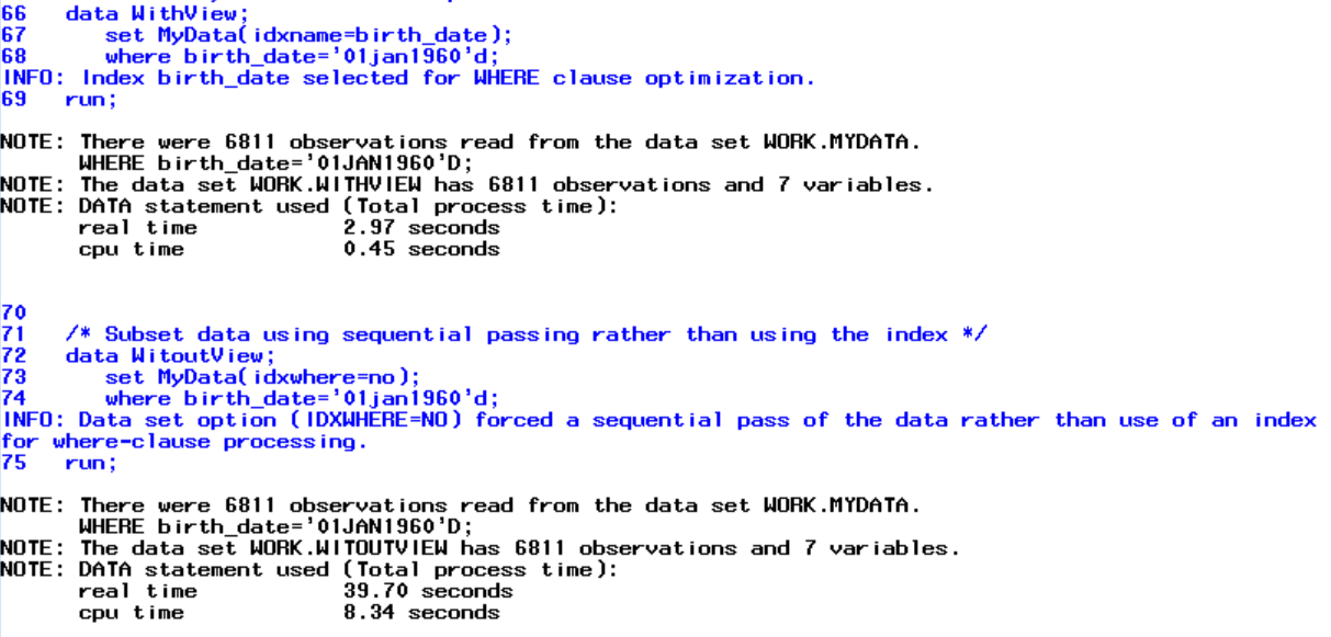
data WithView;
   set MyData(idxname=birth_date);
   where birth_date='01jan1960'd;
run;
 
data WitoutView;
   set MyData(idxwhere=no);
   where birth_date='01jan1960'd;
run;

I have posted my log to the right. The first data step, which uses the index takes 2.97 seconds to run. The second one takes 39.70 seconds. A pretty sizable real time-saving. The use of indexes is not limited to data steps. All procedures and data steps that support the WHERE Statement can take advantage of indexes.

Subsetting data like this is just one way to utilize a SAS index. Another very common way is to use the Data Step Modify Statement and subset conditionally on the _IORC_ Automatic Variable.

Summary

This post demonstrates how the use of indexes on SAS data sets can reduce run time and increase the performance of your code. This post is merely an appetizer to how powerful indexes can be. It is in no way comprehensive. If you are interested, there are dozens of articles out there on the topic. Michael A. Raithel gives a short but comprehensive introduction in the article Creating and Exploiting SAS Indexes. By far the best reference though is the book The Complete Guide to SAS Indexes by the same author. He is also quite fund of PROC DATASETS. In fact, he also wrote the article PROC DATASETS; The Swiss Army Knife of SAS® Procedures.

There are many ways to increase performance in SAS. You can use Hash Object Lookups or Create In Memory Libraries with the MEMLIB Option. Also, see the blog post about Bitmap Searching in SAS. Also, see the blog post The Importance Of SAS Index Centiles.

You can download the entire program from this post here.