In the linear regression model, we explain the linear relationship between a dependent variable  and one or more explanatory variables
  . In matrix notation we write the model as
  . Here, is a vector of dependent variables to be explained.
  is the overall mean of the model.
  is a matrix of independent explanatory variables.
  is a vector of residuals and
  is a vector of parameters to be estimated from the independent variables. In this post, I present an example of how to code linear regression models in SAS.
The usual method of estimating is Ordinary Least Squares (OLS). OLS minimizes the sum of the squared residuals. This method leads to the closed form solution for the estimated parameters ,  . We assume that the error terms have finite variance and are uncorrelated with the regressors. That means the estimator is unbiased and consistent. Further assuming that the variance is constant through the observations, the estimator is also efficient. Wikipedia provides a more thorough examination of the theory of the linear regression model.
Fit a linear regression model in SAS
The simplest way to fit linear regression models in SAS is using one of the procedures, that supports OLS estimation. The first procedure you should consult is PROC REG. A simple example is
proc reg data = sashelp.class; model weight = height; run; |
In the MODEL statement, we list the dependent variable on the left side of the equal sign and the explanatory variables on the right side. This means that the model looks like this

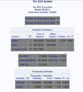
The REG Procedure produces a lot of output and it is important to go about this in the right order. First, you should look at the ‘Fit Diagnostics’ plots. Based on the histogram and QQ plots, does your data look approximately normal? If so, you can proceed to look at the ‘Analysis of Variance’ and ‘Parameter Estimates’. Here, you can see that we get a very small p-value for the overall model. So, the probability of obtaining our data purely by chance is very small. This indicates a good overall model fit. Finally, you should have a look at the parameter estimates and the t-tests and p-values. In this case, both the Intercept and the parameter for Weight are highly significant.
Remember that you can Control Your Output With ODS Select And Exclude if you are not interested in all the procedure output.
The OLS parameter estimates provided by PROC REG imply that the best fitting linear regression model given the specified variables is

which means that a unit of increase in Weight implies a 3.9 unit increase in Height. If an intercept does not make sense in your model, you can suppress it using the NOINT Option in the Model Statement.
Using PROC GLM
The linear regression model is a special case of a general linear model. Here the dependent variable is a continuous normally distributed variable and no class variables exist among the independent variables. Therefore, another common way to fit a linear regression model in SAS is using PROC GLM. PROC GLM does support a Class Statement.
proc glm data = sashelp.class; model weight = height; run; |
For more material and examples of model fitting using the above procedures, consult the SAS documentation for PROC REG and PROC GLM. Both procedures assume normality. Therefore, you should familiarize yourself with the Normal Distribution.
Linear Regression in IML
The two procedures used in the section above produce a lot of output and information with little code. However, it can be a bit confusing how SAS actually calculates these quantities. Therefore, I have written an IML program below, that calculates all the quantities from the ‘Analysis of Variance’ and ‘Parameter Estimates’ sections in the previous. Admittedly, using three lines of code one of the above procedures is much simpler than doing this through IML. However, it gives a nice overview of the calculations performed in linear regression.
proc iml; use sashelp.class; /* Open dataset for reading */ read all var {'weight'} into y; /* Read dependent variable into vector y */ read all var {'height'} into X[c=names];/* Read independent variable(s) into matrix X */ close sashelp.class; /* Close dataset for reading */ df_model = ncol(X); /* Model degress of freedom */ X = j(nrow(X),1,1) || X; /* Intercept */ df_error = nrow(X) - ncol(X); /* Error degrees of freedom */ beta_hat = inv(t(X)*X) * t(X)*y; /* Solve normal equations for parameter estimates */ y_hat = X*beta_hat; /* Predicted values */ res = y - y_hat; /* Residuals */ SSM = sum((y_hat - mean(y))##2); /* Model Sum of Squares */ SSE = sum(res##2); /* Eror Sum of Squares */ MSM = SSM / df_model; /* Model Mean Square */ MSE = SSE / df_error; /* Error Mean Square */ R_square = SSM / (SSM + SSE); /* R^2 */ F = MSM / MSE; /* F test statistic for overall model */ p_F = 1 - CDF('F',F,df_model,df_error); /* p-values */ std_err = sqrt(MSE*vecdiag(inv(t(X)*X))); /* Standard Errors of estimated parameters */ t = beta_hat / std_err; /* t test statistic for estimated parameters */ p_t = 2 * (1-cdf('t',abs(t),df_error)); /* p values for s */ print ('Intercept' // t(names))[l='Parameters'] beta_hat[f=best10.2 l='Estimate'] std_err[f=best10.2 l='Std. Error'] t[f=best5. l='t Value'] p_t[f=pvalue6.4 l='p Value']; /* Print beta values, t-stats and p-values */ print R_square[f=best10.2 l='R^2']; print ({'Model', 'Error', 'Corrected Total'})[l='Source'] (df_model // df_error // df_model+df_error)[f=best10. l='DF'] (SSM // SSE // SSM+SSE)[f=best10. l='Sums of Squares'] (MSM // MSE)[f=best10. l='Mean Square'] F[f=best5. l='F Value'] p_F[f = pvalue6.4 l='p Value']; /* Print sums of squares, F test and p-value */ quit; |
As you can see, the PROC IML code example produces the same results as the previous procedures.
Summary
Summing up, the linear regression model is one of the most common statistical models in introductory statistics courses. Nevertheless, many of the features of the model are essential in other, more complicated models. Therefore, a good understanding of the model will give you an advantage when you fit other classes of linear models.
For further reading, I recommend the book SAS For Linear Models.
Finally, you can download the entire program here.