 . A discrete random variable
  is Poisson distributed with parameter if its Probability Mass Function (PMF) is of the form
If a random variable is Poisson distributed with parameter , this is written as  .
.
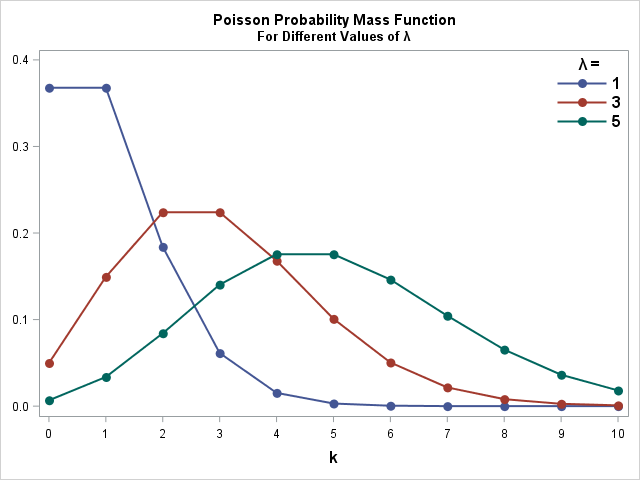
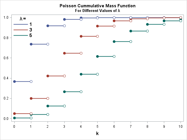
To the right, I plot the Probability Mass Function (PMF) and the corresponding Cumulative Mass Function (CMF). I do so for three different Poisson distributions with parameters  and
and  . The Poisson is a discrete distribution. Therefore, be aware that the lines in the PDF plot is only for comparison of the three densities. Also, the PMF is only defined for integer values of
  . In addition, you can download the program the program creating the plots here.
The Poisson distribution expresses the probability that a given count of events will occur in a given time period, given that these events usually occur with a known constant average rate. Given that you though a whole 24-hour day receive three E-mails per hour on average. What is the probability that in the next hour, you will receive seven E-Mails? This is the question that the Poisson answers. Here, we would set  , since this is the mean of the distribution. Since the mean and variance are the same in the Poisson distribution, the variance will also be equal to 3. Therefore, we can model this example by a stochastic variable
  , which has Probability Mass Function equal to the red function in the PMF plots above.
Poisson Distribution Example SAS Code
It is important to know the shape of the distribution you are working with. Therefore, I have written a small sample code below to play around with the Poisson. Set to different values, run the program and see how the Probability Mass Function changes. What happens when  is large? And what happens when it is small?
%let lambda=4; data Poisson_PMF; do k=0 to 10; PMF=pdf('Poisson', k, &lambda); output; end; run; title "Poisson Probability Mass Function."; title2 "For (*ESC*){unicode lambda} = &lambda."; proc sgplot data=Poisson_PMF noautolegend; vbar k / response=PMF barwidth=0.5 legendlabel="PMF"; keylegend / location=inside position=NE across=1; yaxis display=(nolabel); run; title; |
In conclusion, The Poisson distribution is popular due to its simplicity, but for the same reason, we need some distribution, that can grasp that the mean and variance are not equal. Working with count data you will often see a pattern where the variance is greater than the mean. Consequently, you should familiarize yourself with the Negative Binomial Distribution, which is a natural extension and does not assume equal mean and variance. Finally, I have written about how to fit a Poisson distribution to univariate data in the blog post Fit Discrete Distribution in SAS.