Today is not all about SAS. The class of Regime Switching Log Normal (RSLN) Models is a widely accepted class of models of equity returns. Regime switching models assume that a process switches between regimes randomly, where each regime has a different parameter set and the the probability of changing regime depends solely on the current regime. In this blog post, I will demonstrate how to simulate an RSLN-2 model using SAS IML.
The RSLN-2 Model
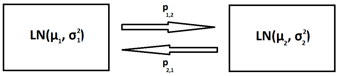 Obviously, in the RSLN-2 case, we switch among
  log-normal models. The switching probabilities
  and
and  denote the probability of switching from regime 1 to 2 and reverse. We let
  denote the regime relevant in the time period from
  to
to  where time is measured in months. Next, let
  be the total value at time and we define
  be the log return process given by
  . Finally, assume that the distribution of the log returns conditional on the regime is given as
  .
.
Maximum Likelihood Model Parameters
A maximum likelihood approach is used in Hardy (2003) to obtain parameters for the RSLN-2 model for the SP500 stock index using a fifty year data window. The parameters are

These are the parameters we use in the simulation Hardy describes the following algorithm to simulate an RSLN-2 model. Before we go to the SAS part, let us review the steps.
- First, draw number
 randomly from uniform distribution .
 - If , then assume that . If not then set
- Generate a standard normal stochastic variate .
- Now let the log-return in the first period of time be given by , which means that the stock price at time is .
- Now draw another from a SAS uniform distribution.
- If , then we assume that . If not, set .
- Repeat steps 3 and forward for desired number of time periods.
- Finally, repeat the preceding steps for the desired number of scenarios
 randomly from uniform distribution
  .
.![u<\mathbb{P}[\rho_0=1]](https://sasnrd.com/wp-content/ql-cache/quicklatex.com-31f80bfb3712cfcec082817dca0b9e80_l3.png "Rendered by QuickLaTeX.com") , then assume that
, then assume that  . If not then set
 .
. , which means that the stock price at time
  is
is ![S_1 = S_0 \exp[Y_1]](https://sasnrd.com/wp-content/ql-cache/quicklatex.com-b1d9a9a2d276bbf9851bf7856c758958_l3.png "Rendered by QuickLaTeX.com") .
. , then we assume that
  . If not, set
  .
.where in step two, we set the probability of the starting regime to be
![\begin{equation*} \mathbb{P} \left[ \rho_0 = 1 \right] = \frac{p_{1,2}}{p_{1,2} + p_{2,1}} \end{equation}](https://sasnrd.com/wp-content/ql-cache/quicklatex.com-20eca837861f34283a397a6717b48f40_l3.png "Rendered by QuickLaTeX.com")
Simulate The Model in SAS
I have implemented the algorithm in a SAS IML Module. Beneath the module, I set up the maximum likelihood parameters and call the module to simulate the RSLN Model.
proc iml; Start RSLN2(per,sce) global(pi_1,spmean, spvar, P); t = t(1:per); /* Vector of time per */ S = j(per,sce,1); /* Vector of Prices */ rho = j(per,1,0); /* Space for regimes */ /* 1. Generate initial Uniform Random Variable */ u = rand("Uniform"); /* 2. If u is less than pi_1 we assume regime 1. */ if u < pi_1 then do; rho[1]=1; mu=spmean[1]; sigma=spvar[1]; end; /* Otherwise we assume that the process is in regime 2.*/ else do; rho[1]=2; mu=spmean[2]; sigma=spvar[2]; end; do j = 1 to sce; do i = 1 to per-1; /* 3. Draw z from standard normal */ z = rand("Normal"); /* 4. Calculate LOG return based on */ /* value of rho and calculate Stock Price */ Y = mu + sigma*z; /* Update Stock Price */ S[i+1,j]=S[i,j]*exp(Y); /* 5. Generate new Uniform Random Variable */ u = rand("Uniform"); /* 6. If the newly generated u is less than the */ /* relevant transition probability, then we */ /* assume that the new regime is 1 */ if (u<(P[rho[i],1])) then do; rho[i+1]=1; mu=spmean[1]; sigma=spvar[1]; end; /* Otherwise we assume regime 2 */ else do; rho[i+1]=2; mu=spmean[2]; sigma=spvar[2]; end; /* 7. Repeat steps 3-7 for desired # periods */ end; /* 8. Repeat steps 1-7 for desired # scenarios */ end; /* Return matrix of Equity Prices S */ S = S || rho; return (S); finish; /* Maximum Likelihood Parameters from Hardy (2003) */ P = {0.9532 0.0468, 0.3232 0.6768}; pi_1 = P[1,2]/(P[1,2]+P[2,1]); spmean = {0.0127, -0.0162}; spvar = {0.0351, 0.1748}; per=100; sce=1; /* Simulate Stockprices */ M = RSLN2(per,sce); VarNames="S1":"S"+char(sce) || "Region"; /* Create Dataset with StockPrice Data */ create StockPrices from M[c=VarNames]; append from M; close StockPrices; quit; |
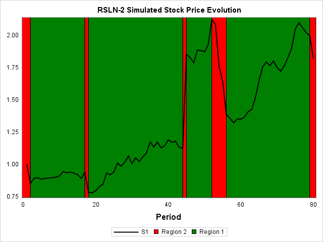
Consequently, you can see the simulated path on the SAS line chart to the left. As expected, we see a more volatile evolution when the process is in regime 2.
Summary
Summing up, the Regime Switching Log Normal model is relatively simple to understand and capture many of the desired properties of equity price evolution. In this post, I demonstrate how to simulate the simplest case with two regimes in SAS PROC IML. Log Normal models are used in many different financial contexts. For example, the Black Scholes Model. Also, check out the blog post Calculate Black Scholes Prices In SAS.
Finally, You can download the entire SAS program from this post, including the graph code here.